Nearshore Sediment Dynamics
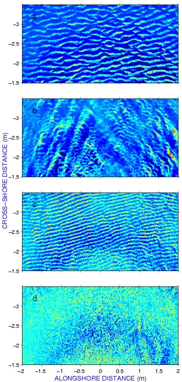
Figure 1:Acoustic images of different bed states. Offshore
is to the top of each panel. High amplitude reflections are yellow and red,
weak signals dark blue. The different bed states are: (a) irregular ripples;
(b) cross ripples; (c) linear transition ripples; and (d) flat bed. From Smyth
et al. (2000).
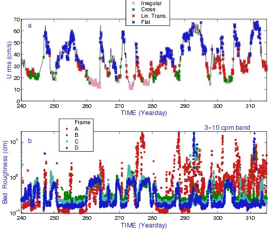
Figure 2: Bed state and rms bottom roughness during SandyDuck97,
determined from rotary fanbeam and pencilbeam
acoustic images of the seabed:
(a) bedstate (irregular ripples, cross ripples, linear transition ripples,
and flat bed); (b) rms bottom roughness in the 3-10 cpm band, at instrument
frames A, B, C, and D located respectively at 65 115 150 and 190 m
distance from the shoreline. The bedstate data in (a) are from
frame C. The results are from Hay and Mudge (2001, manuscript in preparation).
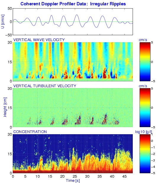
Figure 3: Coherent Doppler Profiler results showing, from top to bottom,
horizontal velocity 20 cm above bottom, vertical velocity in the incident
wave band as a function of height above bottom, vertical velocity in the
turbulence band, and suspended sediment concentration. Irregular ripple
bed state. (from Smyth et al., 2000).
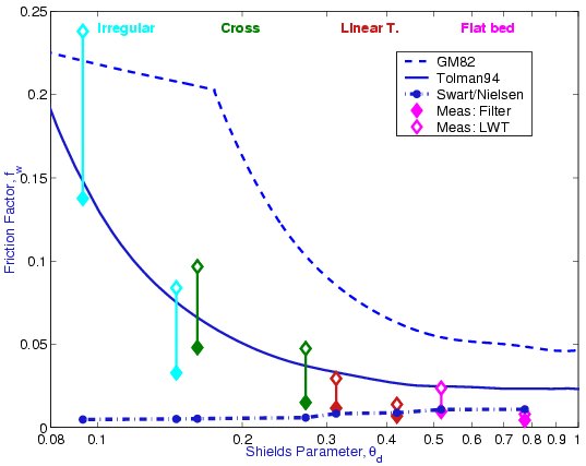
Figure 4: Wave friction factors from 2 nearshore field experiments,
Sandyduck97 and Queensland95, obtained from CDP-measured nearbed
turbulence intensities, for different bed states (irregular ripples, I;
cross ripples, X; linear transition ripples, LT; and flat bed, F) plotted as a
function of grain-roughness Shields parameter (effectively wave energy,
as the grain size was
essentially the same). The vertical lines joining the solid and
open diamonds indicate two different estimators of nearbed turbulence
in the presence of waves. There are two such bars for each ripple type,
one for each experiment, the one at higher Shields parameter being
SandyDuck. The solid line corresponds to Tolman (1994).
(from Smyth et al., 2000, and Smyth and Hay, 2001).

Figure 5: Nearbed maximum intensity of the vertical component of turbulence,
2w'rms (which has been shown in laboratory experiments to be
approximately equal to u*) for different bed states during the
Queensland95 and
Sandyduck97 experiments. From Smyth and
Hay, 2001.

Figure 6: Vertical profiles of the inertial subrange turbulence
spectral slope for different bed states during
Sandyduck97 in: (a) frequency domain; (b) wavenumber space. From Smyth and
Hay, 2001.

Figure 7: Migration velocities (Mr) of linear transition ripples versus
wave orbital velocity skewness. The
solid red circles correspond to storm growth, when migration was negative
offshore); the solid green triangles to storm decay, when migration was
predominantly onshore (from Crawford and Hay, 2001a).
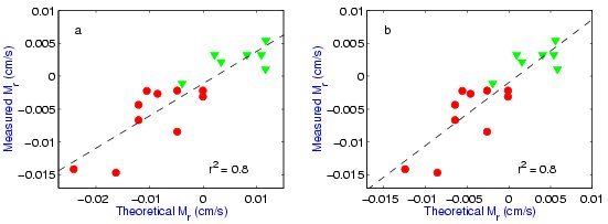
Figure 8: Migration velocities (Mr) of linear transition ripples
versus the theoretical
migration rate estimated from the Meyer-Peter and
Müuller semi-empirical bedload transport formula.
Bed stress estimated using grain roughness and (a) rms orbital
velocity or (b) significant orbital velocity. Dashed line is best fit;
dash-dot line 1:1. Symbols
as in Figure 7. (From Crawford and Hay, 2001b).

Figure 9: Real parts of the bispectra of cross shore velocity during offshore
ripple migration and storm growth (left panel), and onshore migration
and storm decay (right panel). In each panel, the part below the diagonal
is the bispectrum computed from the velocity measured 20 cm above the bed;
the part above the diagonal the bispectrum computed from weakly non-linear
wave theory (From Crawford and Hay, 2001b).
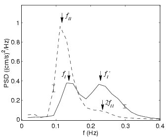
Figure 10: Energy spectra of nearbed cross shore velocity showing the swell
and sea peaks (fI and fI') during
storm growth (solid),
and the swell and its harmonic (fII and
2fII) storm decay (dashed). From Crawford and Hay (2001a).

Figure 11: Comparison between CDP-measured and theoretical vertical
structure of the velocity field above
a flat sloping bed under waves. The bottom slope is 2o.
Top panels are the magnitude and
phase of the horizontal velocity; bottom panels are the magnitude and
phase of the vertical velocity. The data are in blue;
inviscid, horizontal bed theory in green; eddy viscosity, sloping
bottom theory in blue. The plotted quantities are the velocity-surface
elevation transfer function (from Zou and Hay, 2001).
This page last updated November 21, 2001.
Back to
Hay